회귀(Regression): "얼마나?"의 문제
분류(Classification): "무엇인가?"의 문제
>> 예측하려는 값의종류
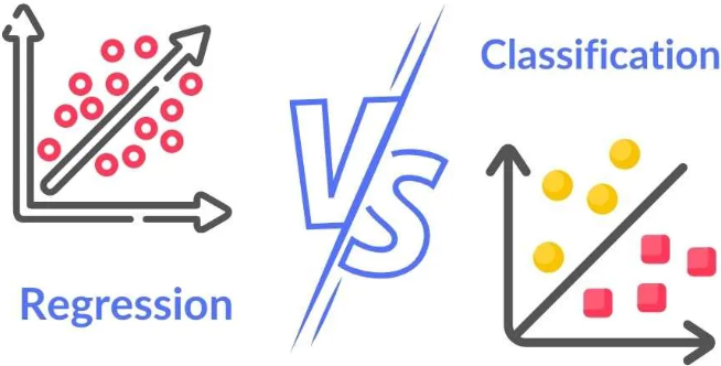
이진 분류(Binary Classification): 2개 클래스 중 하나 선택(0,1/yes,no)
다중 분류(Multi-class Classification): 3개 이상 클래스 중 하나 선택
[실습]타이타닉 생존 예측(분류 문제의 시작)
1. 데이터 불러오기
2. 간단한 분석 해보기
EDA(성별, 생존자)
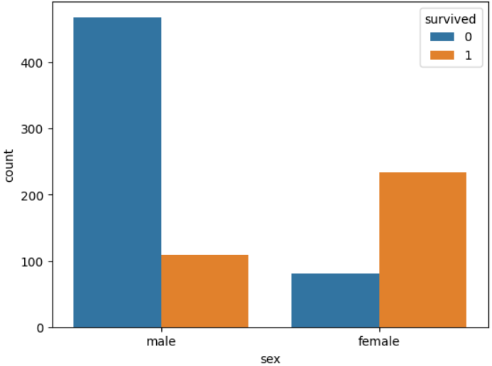
3. 예측하기(여성 생존, 남성 사망)
import pandas as pd

# 결측치 제거 (sex 또는 survived에 NaN이 있는 경우 제외)
titanic = titanic.dropna(subset=['sex', 'survived'])

# 성별 기반 예측
titanic['predicted'] = titanic['sex'].apply(lambda x: 1 if x == 'female' else 0)

# 정확도 계산
accuracy = (titanic['predicted'] == titanic['survived']).mean()
print(f'성별만을 활용한 예측 정확도: {accuracy:.4f}')
로지스틱 회귀 분석
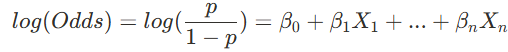
종속변수가 범주형(0, 1)일 때 사용하는 방법
- 시그모이드 함수 사용으로 항상 0~1 사이 값 보장
- S자 곡선 형태로 자연스러운 확률 변화 표현
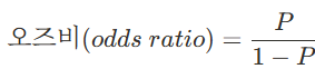
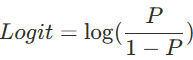
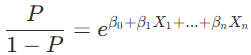
- 3단계 변환 과정: 확률 → 오즈비 → 로짓 → 선형식

β값
- 경사하강법(gradient descent): 오차를 최소화하기위한 값
- 성공 확률 p (X 데이터를 input으로 넣게 된 후)
- 가중치 β, 해당 X 변수의 영향도 파악
- X 변수가 1 증가할 때, exp(해당 β값)만큼 성공확률 상승
Scikit-learn
1. 라이브러리 import
from sklearn.linear_model import LogisticRegression
from sklearn.model_selection import train_test_split
from sklearn.metrics import accuracy_score, classification_report
import pandas as pd
import numpy as np
import seaborn as sns- LogisticRegression: sklearn의 로지스틱 회귀 모델 클래스
- train_test_split: 데이터를 훈련/테스트 세트로 분할하는 함수
- accuracy_score, classification_report: 모델 성능 평가를 위한 함수들
- seaborn: 타이타닉 데이터셋을 쉽게 로드할 수 있는 라이브러리
2. 데이터 준비
# 타이타닉 데이터셋 로드
titanic = sns.load_dataset('titanic')

# 기본 정보 확인
print("데이터셋 기본 정보:")
print(f"전체 데이터 수: {len(titanic)}")
print(f"생존자 수: {titanic['survived'].sum()}")
print(f"생존률: {titanic['survived'].mean():.3f}")
print("\n데이터 샘플:")
print(titanic.head())

# 결측치 확인
print("\n결측치 현황:")
print(titanic.isnull().sum())- sns.load_dataset('titanic'): seaborn에서 제공하는 타이타닉 데이터셋을 로드
- 데이터의 기본 통계 확인: 전체 데이터 수, 생존자 수, 생존률 계산
- head(): 데이터의 첫 5행을 확인하여 데이터 구조 파악
- isnull().sum(): 각 컬럼별 결측치 개수 확인 (전처리 계획 수립을 위해 필수
3. 데이터 전처리
# 데이터 전처리
# 1. 필요한 특성만 선택
features_to_use = ['pclass', 'sex', 'age', 'sibsp', 'parch', 'fare', 'embarked']
titanic_clean = titanic[features_to_use + ['survived']].copy()

# 2. 결측치 처리
titanic_clean['age'] = titanic_clean['age'].fillna(titanic_clean['age'].median())
titanic_clean['fare'] = titanic_clean['fare'].fillna(titanic_clean['fare'].median())
titanic_clean['embarked'] = titanic_clean['embarked'].fillna(titanic_clean['embarked'].mode()[0])

# 3. 범주형 변수 인코딩
titanic_clean['sex'] = titanic_clean['sex'].map({'male': 0, 'female': 1})
titanic_clean = pd.get_dummies(titanic_clean, columns=['embarked'], prefix='embarked', drop_first=True)

# 독립변수와 종속변수 분리
X = titanic_clean.drop('survived', axis=1)
y = titanic_clean['survived']

print("전처리 완료!")
print(f"특성 수: {X.shape[1]}")
print(f"특성 목록: {list(X.columns)}")
print("\n전처리된 데이터:")
print(X.head())- 특성 선택: 생존 예측에 유의미한 특성들만 선별 (deck, who 등은 제외)
- 결측치 처리:
- 수치형 변수(age, fare): 중앙값으로 대체 (이상치에 덜 민감)
- 범주형 변수(embarked): 최빈값으로 대체
- 범주형 변수 인코딩:
- sex: 수동 매핑 (male=0, female=1)
- embarked: 원-핫 인코딩 (drop_first=True로 다중공선성 방지)
- 변수 분리: 독립변수(X)와 종속변수(y)로 분리하여 모델 학습 준비
4. 모델 생성 및 학습
# 훈련/테스트 데이터 분할
X_train, X_test, y_train, y_test = train_test_split(X, y, test_size=0.2, random_state=42, stratify=y)

# 로지스틱 회귀 모델 생성
model = LogisticRegression(random_state=42, max_iter=1000)

# 모델 학습
model.fit(X_train, y_train)

print("모델 학습 완료!")
print(f"계수(coefficients): {model.coef_[0]}")
print(f"절편(intercept): {model.intercept_[0]:.3f}")- train_test_split: 데이터를 8:2 비율로 분할, stratify=y로 클래스 비율 유지
- LogisticRegression: 기본 파라미터로 모델 생성
- fit(): 훈련 데이터로 모델 학습 수행
- 학습된 모델의 계수와 절편 출력하여 각 특성의 영향력 확인
5. LogisticRegression 메서드
# 다양한 하이퍼파라미터 설정 예시
model_detailed = LogisticRegression(
    penalty='l2',# 정규화 방법
    C=1.0,# 정규화 강도의 역수
    solver='lbfgs',# 최적화 알고리즘
    max_iter=1000,# 최대 반복 횟수
    tol=1e-4,# 수렴 임계값
    fit_intercept=True,# 절편 포함 여부
    class_weight=None,# 클래스 가중치
    random_state=42# 난수 시드
)
6. 모델 성능 평가
# 테스트 데이터로 예측
y_pred_train = model.predict(X_train)
y_pred_test = model.predict(X_test)

# 정확도 계산
train_accuracy = accuracy_score(y_train, y_pred_train)
test_accuracy = accuracy_score(y_test, y_pred_test)

print(f"훈련 데이터 정확도: {train_accuracy:.3f}")
print(f"테스트 데이터 정확도: {test_accuracy:.3f}")

# 상세한 분류 보고서
print("\n=== 테스트 데이터 분류 보고서 ===")
print(classification_report(y_test, y_pred_test, target_names=['사망', '생존']))- 훈련/테스트 정확도 비교: 과적합 여부 확인
- 훈련 정확도 >> 테스트 정확도: 과적합 의심
- 두 정확도가 비슷: 적절한 일반화 성능
- classification_report(): 정밀도, 재현율, F1-score 등 상세 성능 지표 제공
- 정밀도(Precision): 생존 예측 중 실제 생존 비율
- 재현율(Recall): 실제 생존자 중 올바르게 예측한 비율
- F1-score: 정밀도와 재현율의 조화평균
- macro avg: 각 클래스별 지표의 단순 평균
- weighted avg: 클래스별 샘플 수를 고려한 가중 평균
7. 모델 학습 결과 해석하기
# 모델 계수 분석
feature_names = X.columns
coefficients = model.coef_[0]

print("=== 타이타닉 생존에 영향을 미치는 요인 분석 ===")
coef_df = pd.DataFrame({
    'Feature': feature_names,
    'Coefficient': coefficients,
    'Odds_Ratio': np.exp(coefficients)
}).sort_values('Coefficient', ascending=False)

print(coef_df)
print("\n=== 상세 해석 ===")
for feature, coef in zip(feature_names, coefficients):
    odds_ratio = np.exp(coef)
    print(f"{feature}: 계수 {coef:.3f}")

    if coef > 0:
        print(f"  → 이 변수가 1단위 증가하면 생존 오즈비가 {odds_ratio:.3f}배 증가")
        print(f"  → 생존에 긍정적인 영향")
    else:
        print(f"  → 이 변수가 1단위 증가하면 생존 오즈비가 {odds_ratio:.3f}배 감소")
        print(f"  → 생존에 부정적인 영향")
    print()
평가 지표
혼동행렬(Confusion Matrix)
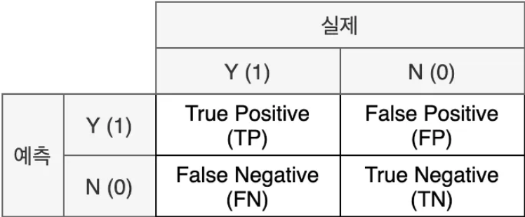
- 실제와 예측이 같으면 True / 다르면 False
- 예측을 양성으로 했으면 Positive / 음성으로 했으면 Negative
[해석]
- TP: 실제로 양성(암 환자)이면서 양성(암 환자) 올바르게 분류된 수
- FP: 실제로 음성(정상인)이지만 양성(암 환자)로 잘못 분류된 수
- FN: 실제로 양성(암 환자)이지만 음성(정상인)로 잘못 분류된 수
- TN: 실제로 음성(정상인)이면서 음성(정상인)로 올바르게 분류된 수
from sklearn.metrics import confusion_matrix, ConfusionMatrixDisplay
import matplotlib.pyplot as plt

import matplotlib.font_manager as fm
#window
plt.rcParams['font.family'] = 'Malgun Gothic'
#mac
plt.rcParams['font.family'] = 'AppleGothic'

# 혼동행렬 계산
cm = confusion_matrix(y_test, y_pred_test)

print("=== 타이타닉 생존 예측 혼동행렬 ===")
print("혼동행렬:")
print(cm)
print(f"\nTrue Negative (정확한 사망 예측): {cm[0,0]}명")
print(f"False Positive (잘못된 생존 예측): {cm[0,1]}명")
print(f"False Negative (잘못된 사망 예측): {cm[1,0]}명")
print(f"True Positive (정확한 생존 예측): {cm[1,1]}명")

# 혼동행렬 시각화
plt.figure(figsize=(8, 6))
disp = ConfusionMatrixDisplay(confusion_matrix=cm, display_labels=['사망', '생존'])
disp.plot(cmap='Blues', values_format='d')
plt.title('타이타닉 생존 예측 혼동행렬', fontsize=14)
plt.show()
지표
1. 정밀도: 거짓 양성 비용이 높을 때(틀렸을 때 매우 큰 손실)

tn, fp, fn, tp = cm.ravel()
precision_manual = tp / (tp + fp)

print(f"타이타닉 생존 예측 정밀도: {precision_manual:.3f}")
2. 재현율: 거짓 음성 비용이 높을 때(맞은 것을 놓치면 안됌)
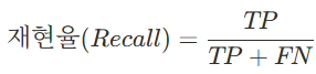
recall_manual = tp / (tp + fn)

print(f"타이타닉 생존 예측 재현율: {recall_manual:.3f}")
>>Trade-off 관계
3. f1-score: 두 개의 조화평균
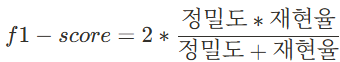
f1_manual = 2 * (precision_manual * recall_manual) / (precision_manual + recall_manual)

print("=== F1-Score===")
print(f"F1-Score: {f1_manual:.3f}")
4. 정확도
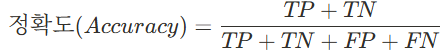
tn, fp, fn, tp = cm.ravel()
accuracy_manual = (tp + tn) / (tp + tn + fp + fn)
accuracy_sklearn = accuracy_score(y_test, y_pred_test)

print(f"수동 계산 정확도: {accuracy_manual:.3f}")
print(f"sklearn 정확도: {accuracy_sklearn:.3f}")
print(f"전체 {len(y_test)}명 중 {tp + tn}명을 정확히 예측했습니다.")
ROC 커브란?
모든 임계값에서의 모델 성능을 한눈에 보여주는 시각화 도구
- X축: False Positive Rate (FPR) = FP / (FP + TN)
- 실제 음성인 것들 중에서 모델이 양성이라고 잘못 예측한 비율
- Y축: True Positive Rate (TPR) = TP / (TP + FN) = Recall
- 실제 양성인 것들 중에서 모델이 양성이라고 올바르게 예측한 비율
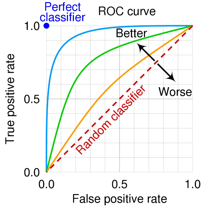
[이상적인 ROC 커브]
왼쪽 상단 모서리에 가까울수록
대각선(랜덤)보다 위에 존재
[중요한 이유]
- 임계값 독립적: 다양한 임계값에서의 성능을 모두 고려
- 모델 비교 용이: 여러 모델의 성능을 한 그래프에서 비교 가능
- 비즈니스 의사결정: TPR과 FPR 트레이드오프를 고려한 임계값 선택
[코드]
1. ROC 커브 그리기
from sklearn.metrics import roc_curve, roc_auc_score, RocCurveDisplay
# 예측 확률 구하기
y_pred_proba = model.predict_proba(X_test)[:, 1] # 생존 확률만 추출
# ROC 커브 데이터 계산
fpr, tpr, thresholds = roc_curve(y_test, y_pred_proba)
roc_auc = roc_auc_score(y_test, y_pred_proba)
RocCurveDisplay.from_estimator(model, X_test, y_test)
plt.title('ROC 커브 (sklearn 제공)')
plt.grid(True)
plt.tight_layout()
plt.show()
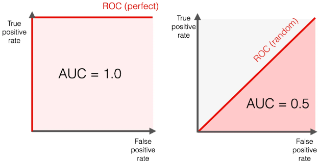
print(f"=== ROC AUC 분석 ===")
print(f"AUC Score: {roc_auc:.3f}")
print()
print("AUC 해석:")
if roc_auc >= 0.9:
print("🌟 탁월한 모델 (0.9-1.0)")
elif roc_auc >= 0.8:
print("✅ 우수한 모델 (0.8-0.9)")
elif roc_auc >= 0.7:
print("⚠️ 준수한 모델 (0.7-0.8)")
elif roc_auc >= 0.6:
print("🔄 개선 필요 (0.6-0.7)")
else:
print("❌ 불량한 모델 (0.5-0.6)")2. 임계값 성능 분석
# 다양한 임계값에서의 성능 분석
# 주요 임계값들에서 성능 계산
thresholds_to_test = [0.3, 0.4, 0.5, 0.6, 0.7]

results = []
for threshold in thresholds_to_test:
    y_pred_custom = (y_pred_proba >= threshold).astype(int)

    # 혼동행렬 계산
    tn, fp, fn, tp = confusion_matrix(y_test, y_pred_custom).ravel()

    # 지표 계산
    accuracy = (tp + tn) / (tp + tn + fp + fn)
    precision = tp / (tp + fp) if (tp + fp) > 0 else 0
    recall = tp / (tp + fn) if (tp + fn) > 0 else 0
    f1 = 2 * precision * recall / (precision + recall) if (precision + recall) > 0 else 0
    fpr = fp / (fp + tn) if (fp + tn) > 0 else 0

    results.append({
        'Threshold': threshold,
        'Accuracy': accuracy,
        'Precision': precision,
        'Recall': recall,
        'F1': f1,
        'FPR': fpr
    })

# 결과를 DataFrame으로 정리
results_df = pd.DataFrame(results)
print(results_df.round(3))

# 최적 임계값 찾기 (F1-Score 기준)
best_threshold_idx = results_df['F1'].idxmax()
best_threshold = results_df.loc[best_threshold_idx, 'Threshold']
best_f1 = results_df.loc[best_threshold_idx, 'F1']

print(f"\n🎯 최적 임계값 (F1-Score 기준): {best_threshold}")
print(f"   최고 F1-Score: {best_f1:.3f}")
'특강 > 머신러닝' 카테고리의 다른 글
| [머신러닝 주요기법] 3회차 (07.02)☆elbow, silhouette (2) | 2025.07.02 |
|---|---|
| [머신러닝 주요기법] 2회차 (07.01) (2) | 2025.07.01 |
| [머신러닝] 4회차 앙상블, 부스팅(06.27) (2) | 2025.06.27 |
| [머신러닝] 3회차 회귀분석 (06.26) (0) | 2025.06.26 |
| [머신러닝] 2회차 머신러닝 핵심기술(06.25) (2) | 2025.06.25 |